2018-07-22

Q太郎

一匹の妖怪がIT産業を徘徊している――量子コンピューターという妖怪が。

というわけで、将来は立派なおばけになりたい私としても量子コンピューターに触れておきたい。
丁度、IBM Q Experience のように無料で 量子コンピューターを利用できるサービス (実行回数制限あり) もあるので、早速始めてみる。

と言いたいのだけれど、そう思い立った頃は PC を買い換えようかと考えていたので、一生懸命環境構築 したところで、すぐに環境を捨ててしまうことになる。

できるだけ手間いらずにしたい。こういう時は Web 上の IDE を使うのが一番。早速 Cloud9 を開く。

https://c9.io


Cloud9、Amazon に買収されてた。

おのれー、Exit おめでとうございます💢
まあいいや、さくっと環境を作ってしまおう。

どれ?


えーっと。

もー!もー!手軽に開発環境を用意できるのが良かったのに、めんどくさーい!

作成完了


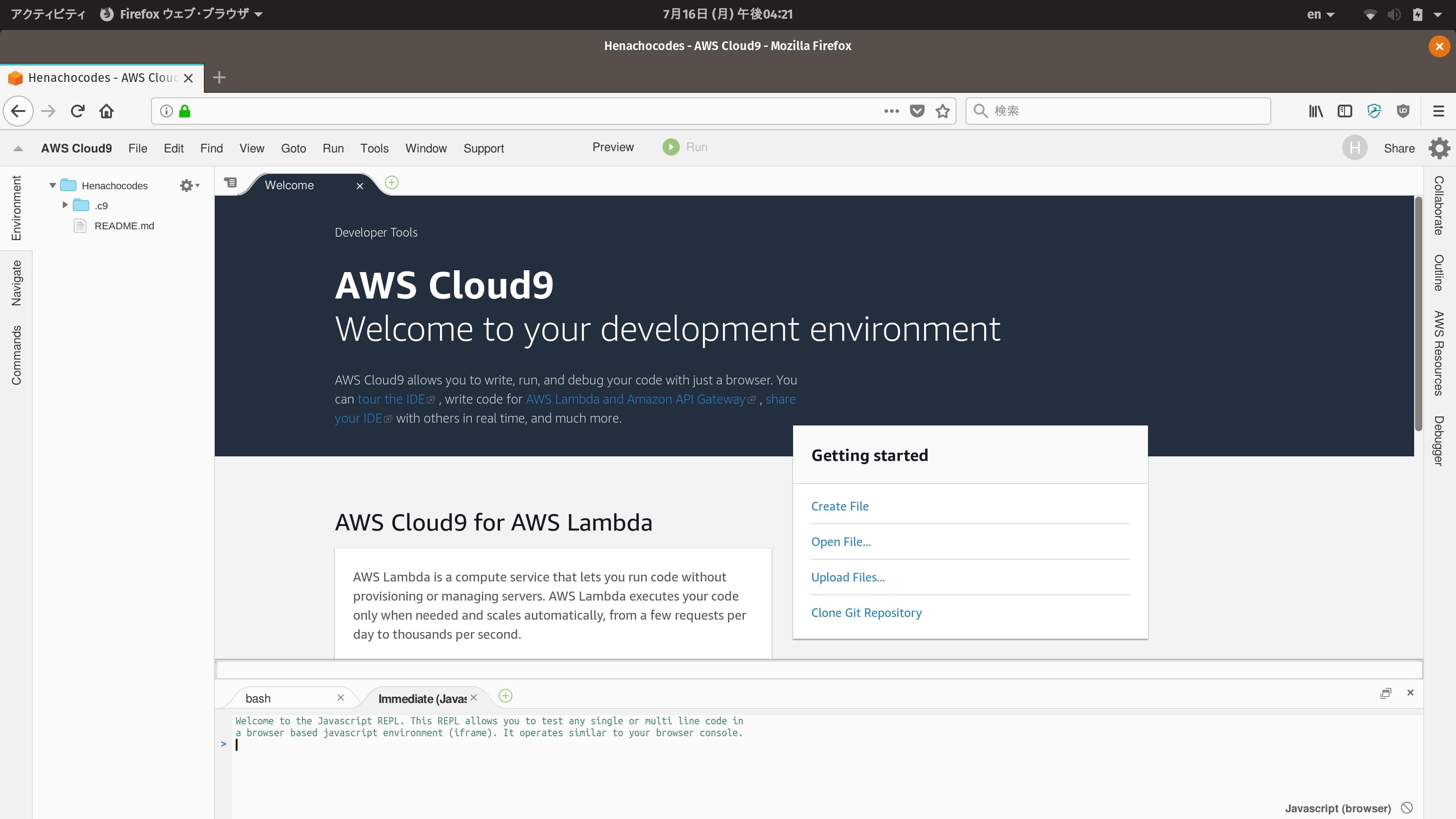
どうにか環境を用意できたので、IBM Q の実行環境を構築し始める。
まずは Python 3 を使うために AWS Cloud9 の Python サンプル を参考にして virtualenv の仮想環境を構築してから切り替える。

$ unalias python
$ cd ~/environment/
$ virtualenv -p /usr/bin/python36 ibmq
$ source ibmq/bin/activate


次に pip で Qiskit をインストールする。

$ pip install qiskit


これで ローカルシミュレーター上でのプログラムの実行はできるようになったので、~/environment の配下に ibmq_sample というディレクトリを作ってから、qiskit_sample.py というファイルを作って、 Qiskit documentation の Getting Started の最初に書いてあるコードをコピペする。

# 仮想環境のディレクトリ名、なんか別のにしとけばよかったな。

qiskit_sample.py を作成


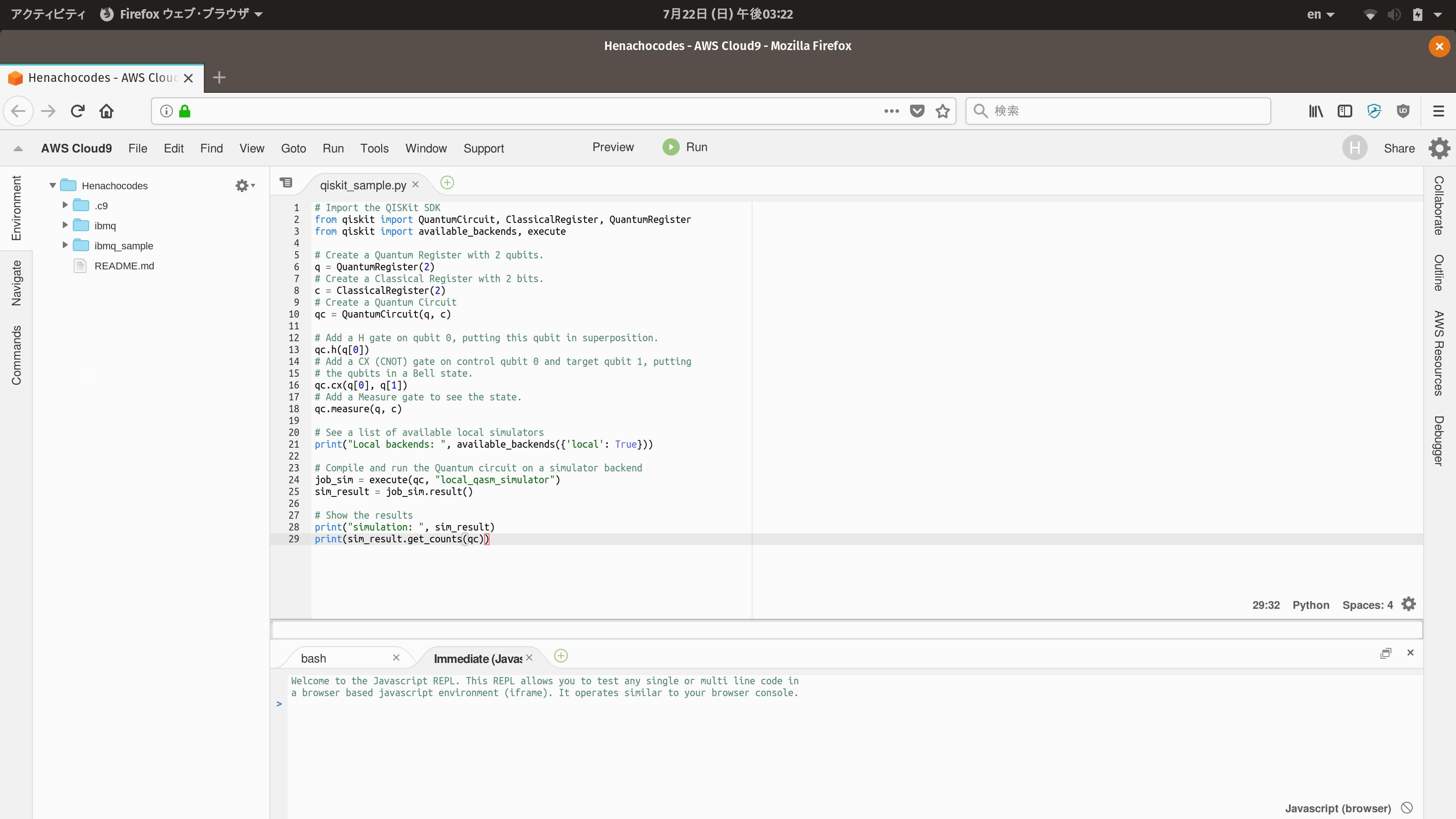
qiskit_sample.py を保存したら、実行する。バケラッタ!(実行の意)

$ python qiskit_sample.py


正常に実行できれば、こんな感じの結果が出力されるはず。

{'00': 525, '11': 499}


サンプルプログラムは get_counts メソッドが返した辞書オブジェクトをそのまま画面に表示していて、キーが結果として 得られた古典ビット列、 値が対応する古典ビット列の出現回数になっている。量子コンピューターの出力は結果とその 確率のペアらしいので、多分それを表現しているんだろう。

せっかくだからシミュレーターだけじゃなくて、実機でも実行してみたい。
というわけで、Qiskit のチュートリアルから適当なプログラムをコピペする。

ここで一つ問題が。
Qiskit のチュートリアルに載ってるサンプルプログラムの多くは、結果を柱状グラフで表示するのだけれど、 この柱状グラフが別ウィンドウで表示されてしまう。

ローカルの環境であれば特に問題はないが、今回は横着して Cloud9 を使ったのでグラフが出てこない。 というわけで、Qiskit の plot_histogram を改変して plot_histogram_file.py を作成し、グラフをファイルに出力する。

 1
 2
 3
 4
 5
 6
 7
 8
 9
10
11
12
13
14
15
16
17
18
19
20
21
22
23
24
25
26
27
28
29
30
31
32
33
34
35
36
37
38
39
from collections import Counter

import matplotlib
matplotlib.use('Agg')
import matplotlib.pyplot as plt
import numpy as np
from scipy import linalg as la

def plot_histogram_file(filename, data, number_to_keep=False):
    """Plot a histogram of data.
    data is a dictionary of  {'000': 5, '010': 113, ...}
    number_to_keep is the number of terms to plot and rest is made into a
    single bar called other values
    """
    if number_to_keep is not False:
        data_temp = dict(Counter(data).most_common(number_to_keep))
        data_temp["rest"] = sum(data.values()) - sum(data_temp.values())
        data = data_temp

    labels = sorted(data)
    values = np.array([data[key] for key in labels], dtype=float)
    pvalues = values / sum(values)
    numelem = len(values)
    ind = np.arange(numelem)  # the x locations for the groups
    width = 0.35  # the width of the bars
    fig, ax = plt.subplots()
    rects = ax.bar(ind, pvalues, width, color='seagreen')
    # add some text for labels, title, and axes ticks
    ax.set_ylabel('Probabilities', fontsize=12)
    ax.set_xticks(ind)
    ax.set_xticklabels(labels, fontsize=12, rotation=70)
    ax.set_ylim([0., min([1.2, max([1.2 * val for val in pvalues])])])
    # attach some text labels
    for rect in rects:
        height = rect.get_height()
        ax.text(rect.get_x() + rect.get_width() / 2., 1.05 * height,
                '%f' % float(height),
                ha='center', va='bottom')
    fig.savefig(filename)


なんか、ほとんど plot_histogram のまんまだし、Python もよく知らないから行儀のいい書き方かどうか 怪しいけど、これでグラフがファイルに出力されるはず。

そいでもって、サンプルプログラムから呼び出すメソッドを plot_histogram_file に変えておく。
ここでは、チュートリアルの 1. Hello, Quantum World に載ってるプログラムを改変する。

 1
 2
 3
 4
 5
 6
 7
 8
 9
10
11
12
13
14
15
16
17
18
19
20
21
22
23
24
25
26
27
28
29
30
31
32
33
34
35
36
37
38
39
40
41
42
43
44
import getpass, time
from qiskit import ClassicalRegister, QuantumRegister, QuantumCircuit
from qiskit import available_backends, execute, register, least_busy

# import basic plot tools
#from qiskit.tools.visualization import circuit_drawer
from plot_histogram_file import *

APItoken = getpass.getpass('Please input your token and hit enter: ')
qx_config = {
    "APItoken": APItoken,
    "url":"https://quantumexperience.ng.bluemix.net/api"}

try:
    register(qx_config['APItoken'], qx_config['url'])

    print('\nYou have access to great power!')
    print(available_backends({'local': False, 'simulator': False}))
except: 
    print('Something went wrong.\nDid you enter a correct token?')

backend = least_busy(available_backends({'simulator': False, 'local': False}))
print("The least busy backend is " + backend)

q = QuantumRegister(2)
c = ClassicalRegister(2)
qc = QuantumCircuit(q, c)
qc.h(q[0])
qc.cx(q[0], q[1])
qc.measure(q, c)
job_exp = execute(qc, backend=backend, shots=1024, max_credits=3)

lapse = 0
interval = 30
while not job_exp.done:
    print('Status @ {} seconds'.format(interval * lapse))
    print(job_exp.status)
    time.sleep(interval)
    lapse += 1
print(job_exp.status)

plot_histogram_file("result.svg", job_exp.result().get_counts(qc))

print('You have made entanglement!')


あと、6行目の circuit_drawer はなんかエラーになるし、とりあえず不要なのでコメントアウトする。
それから、ファイル名を hello_quantum_world.py として保存する。

ソースコードを保存したら、IBM Q Experience にログインして、APIトークンを発行してから実行する。

$ python hello_quantum_world.py


実行するとAPIトークンを聞かれるので入力する。

Please input your token and hit enter:


何回かエラーが返ってくることがあるけれども、気にせずにプログラムの終了を待つと、

You have access to great power!
['ibmqx2', 'ibmqx4', 'ibmqx5']
The least busy backend is ibmq_5_tenerife
Status @ 0 seconds
{'job_id': None, 'status': <JobStatus.INITIALIZING: 'job is being initialized'>,
'status_msg': 'Job is initializing. Please, wait a moment.'}
{'job_id': '5b5428fe221a72003943d00f', 'status': <JobStatus.DONE: 'job has successfully run'>,
'status_msg': 'job has successfully run'}
You have made entanglement!


結果が返ってくる。
(ここの実行結果例は読みやすいようにエラー出力を省略して、さらに途中で改行している)

# available_backends の結果がチュートリアルと全然違うのが気になる。なんか間違えてるかな。

で、プログラムの実行が正常に終了していれば、result.svg というファイルがソースコードと同一の ディレクトリに出力されているので、ダウンロードして開いてみると、
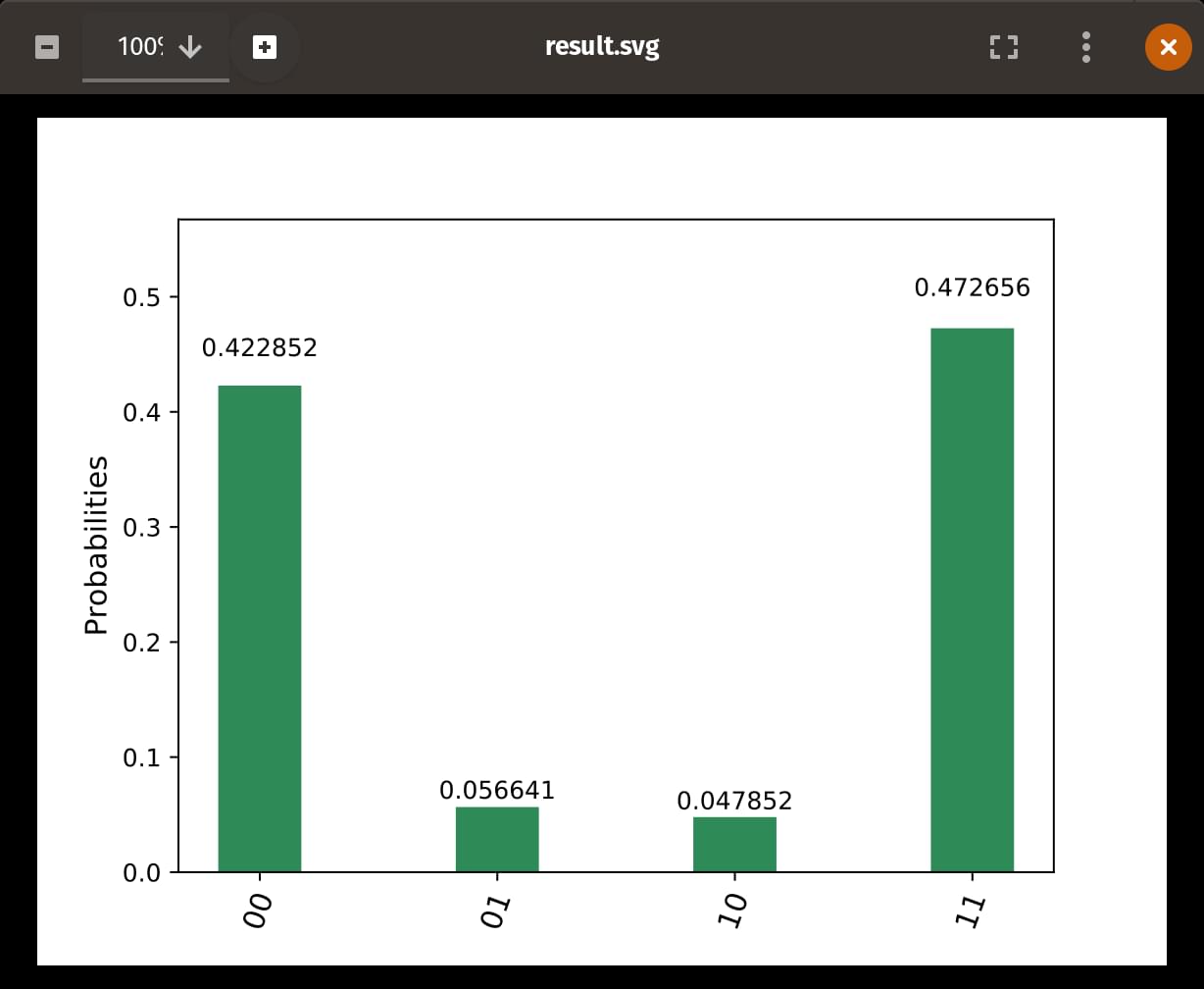
hello_quantum_world.py の実行結果


こんな感じのグラフが出てくる。 シミュレーターと違って実機の場合はノイズがあるので、 “00”、 “11” 以外の結果も出てくる。

とここまで、Cloud9 で IBM Q を動かしてみる方法を書いてみたものの、久々に試してみたらやたらと エラーが出まくるし、Qiskit は名前からして変わってるしで何だかもやもやする。

あれか、妖怪のしわざってやつか。

ホームへ戻る